Intro to Maps
and Spatial
Data

Day 05

Prof Amanda Luby

Carleton College
Stat 220 - Winter 2026

Today

  • git/GitHub
  • Intro to Spatial Data
  • Making Maps in ggplot2

  • Think of the state on GitHub as “worst case scenario”
  • If you screw things up, copy your important files (eg. hw02.qmd) to a safe place.
    • Usually your files are JUST FINE. But it is easy to goof up the Git infrastructure when you’re new at this. And it can be hard to get that straightened out on your own.
  • Rename the existing local repo as a temporary measure, i.e. before you do something radical, like delete it.
  • Clone the original repo from GitHub to RStudio (follow the directions to create a new project). You are back to a happy state.
  • Copy all relevant files back over from your safe space. The ones whose updated state you need to commit.
  • Knit, commit, push
  • Carry on with your life.

Spatial Data

Cholera

In 1854, a Cholera outbreak killed 127 people in 3 days in a London neighborhood, resulting in a mass exodus of local residents. At the time, people thought that Cholera w as an airborne disease. John Snow was a physician who was critical of the airborne theory, and set out to investigate.

What might this data look like?

date last_name first_name address age cause_of_death
Aug 31, 1854 Jones Thomas 26 Broad St. 37 cholera
Aug 31, 1854 Jones Mary 26 Broad St. 11 cholera
Sept 1, 1854 Warwick Martin 14 Broad St. 23 cholera

What makes “address” a useful variable is that it is linked to a specific location in the physical world. If we plot these addresses, we get something like the following:
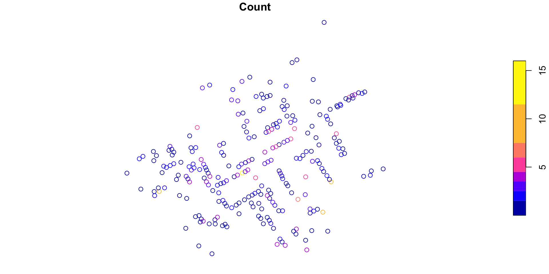
While we can see patterns in the last plot, the underlying map of the London streets provides helpful context that makes it more intelligble:
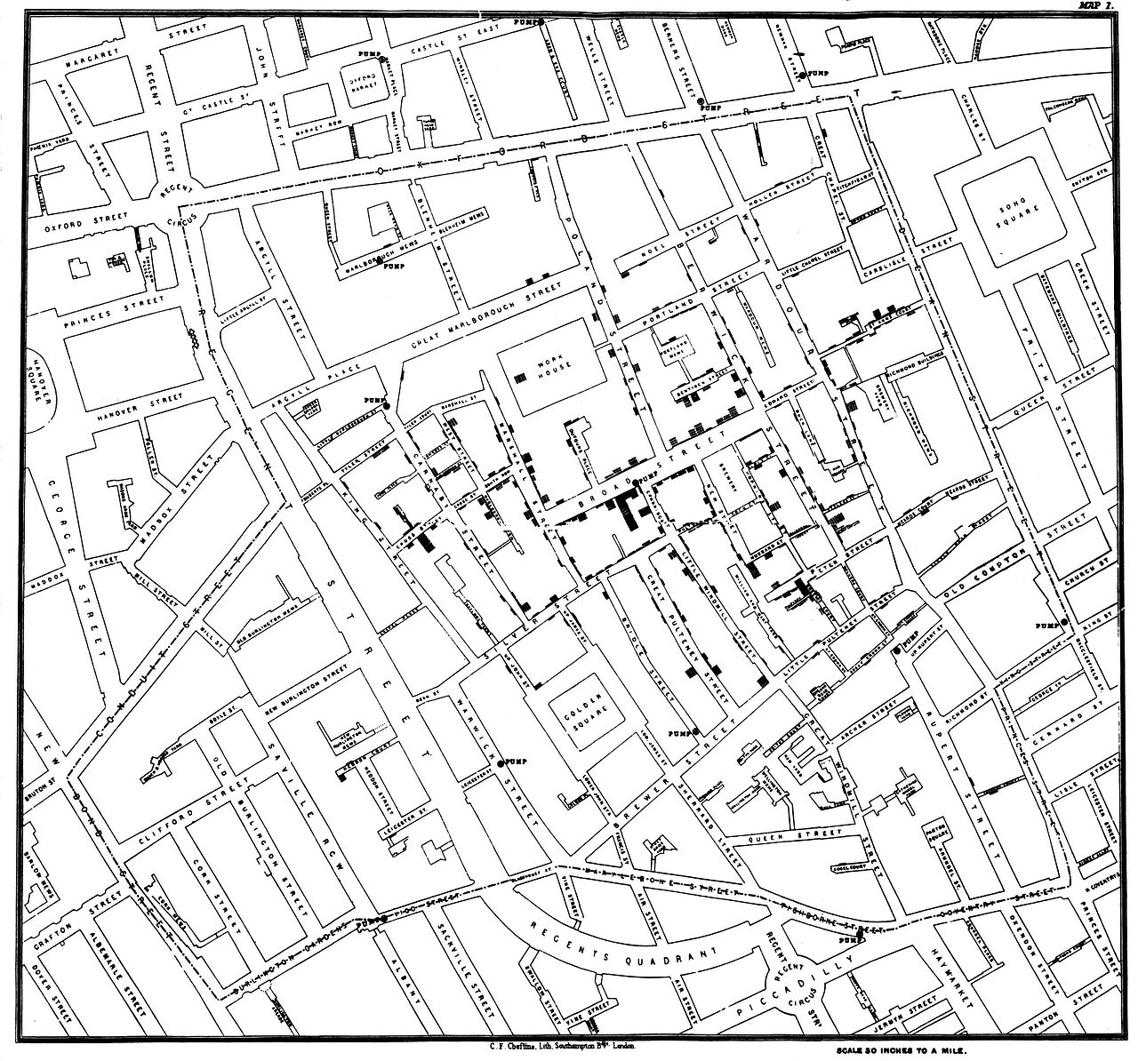
Snow’s insight was driven by another set of data—the locations of the street-side water pumps (it’s kind of hard to see, but they are labelled on the map). Nearly all of the cases were clustered around a single pump on the center of Broad Street.

John Snow’s map (and water pump) are now “famous” among epidemiologists and statisticians.

John Snow’s water pump (and pub) from a 2019 visit

A successful data science episode:

  1. Combine three sources of data (Cholera deaths, water pump locations, and street map)
  2. While a model might have come to the same conclusion, simply plotting the data is much simpler (and more convincing to lots of people)
  3. The problem was resolved when the data-based evidence was combined with a plausible model that explained the physical phenomenon.

Common Types of Maps

  1. Chloropleth
  2. Proportional Symbol
  3. Cartograms/Geofacets

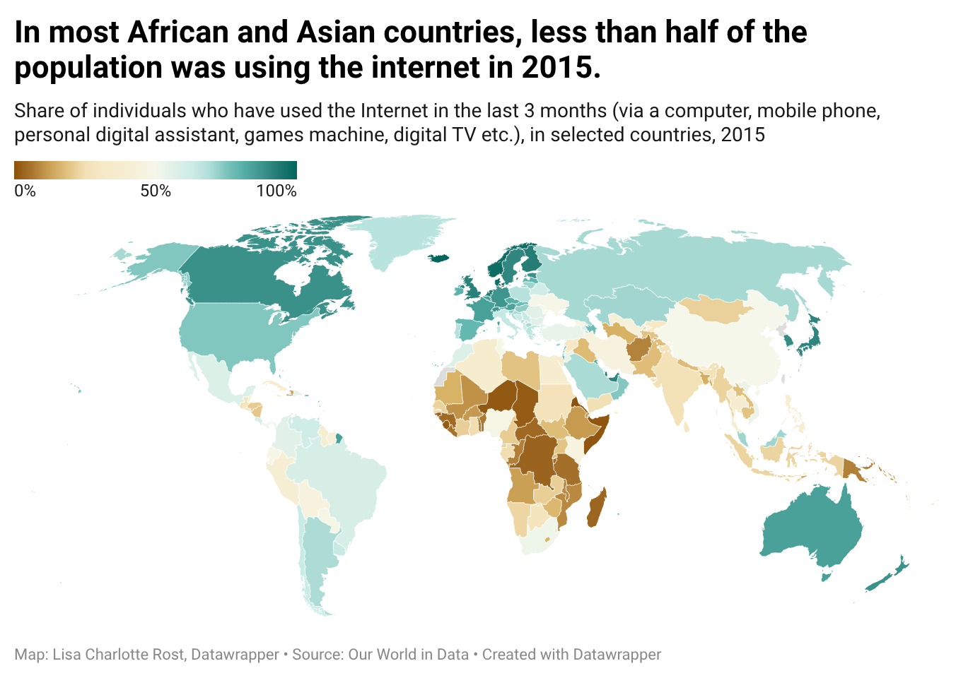
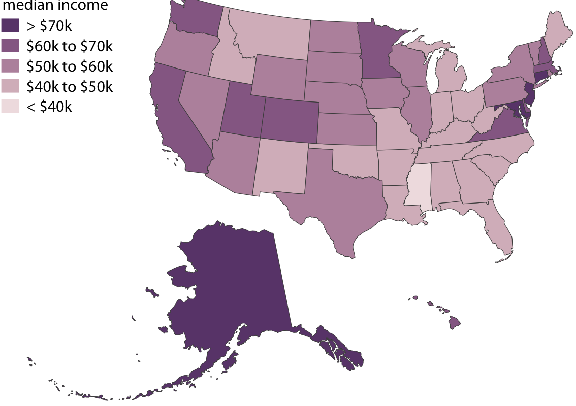
Chloropleth

Fill in regions with variable values

Need two data sources:

  1. map data with lat, long, region
  2. data with measurements for each region
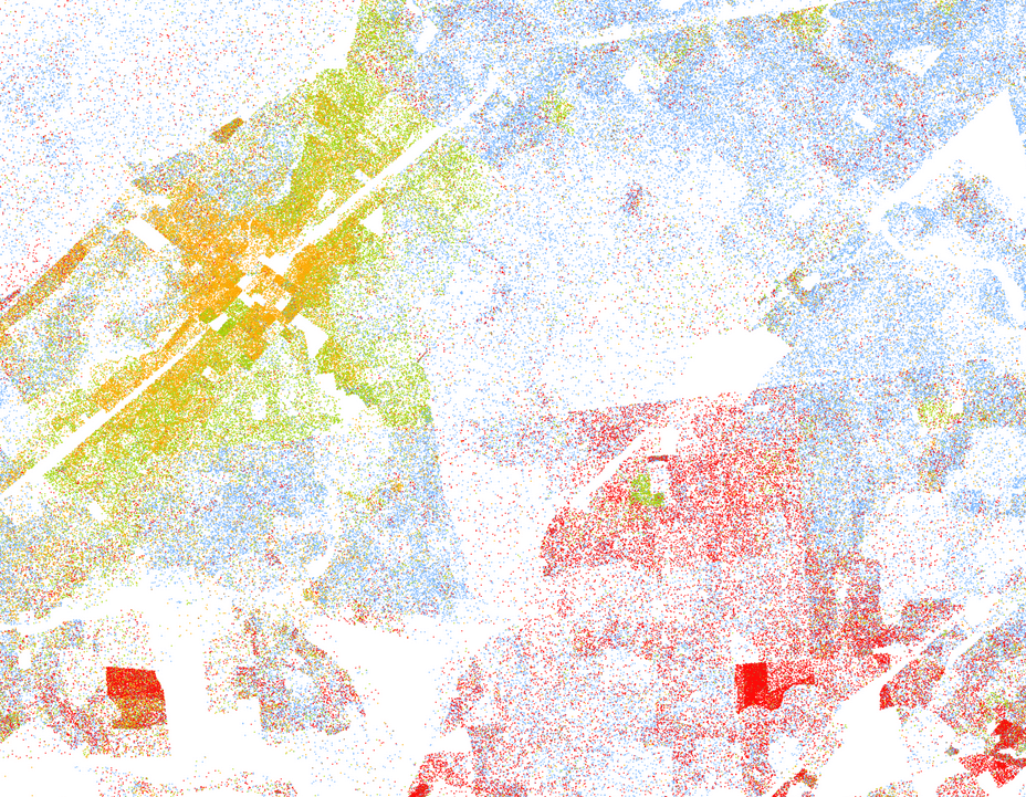
Dot density

Uses points to show distribution and concentration, where each dot represents a specific quantity. Here 1 dot = 1 person:
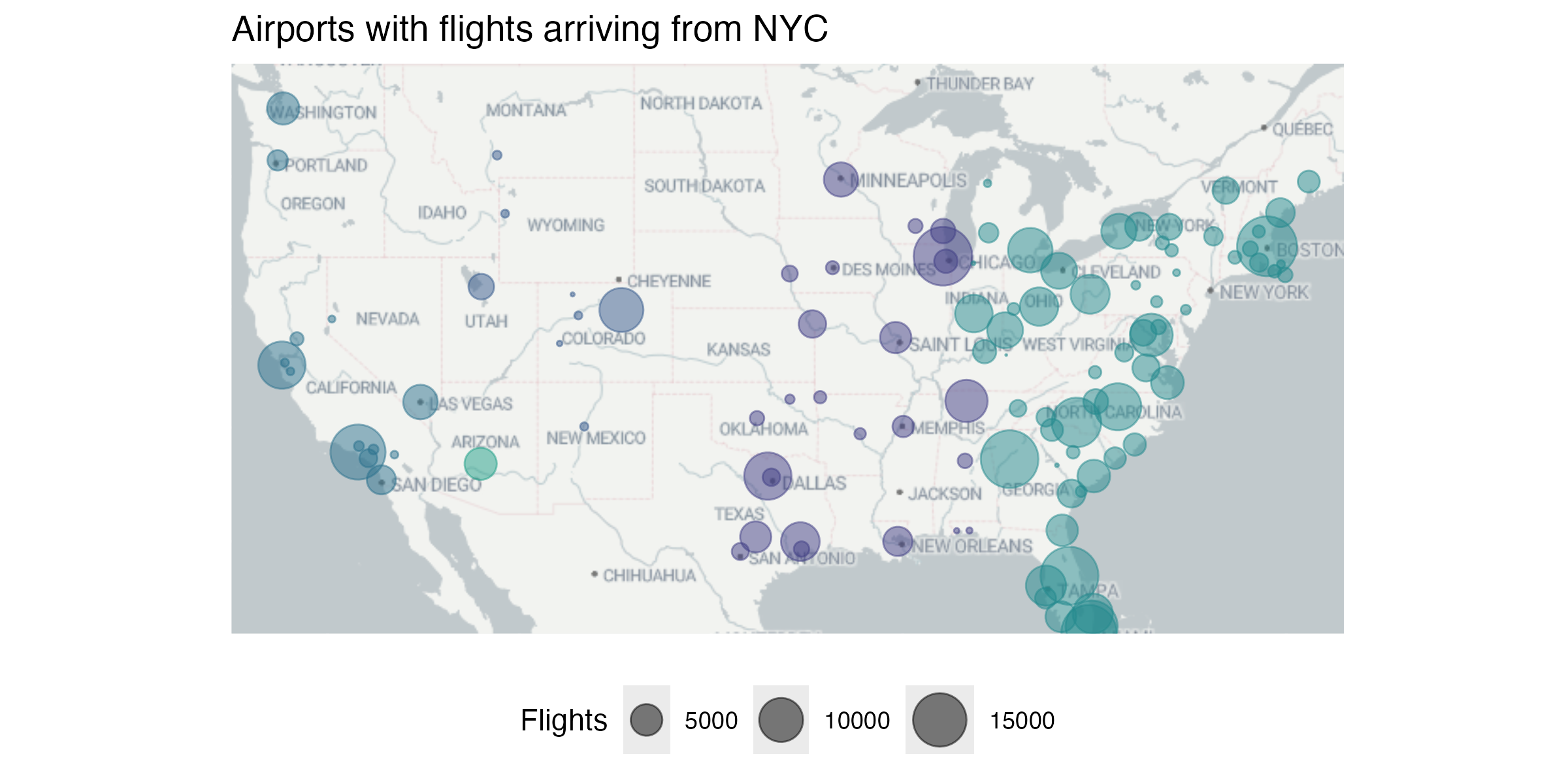
Proportional Symbol

Overlay symbols on an existing map, where the size of the shape is proportional to the variable
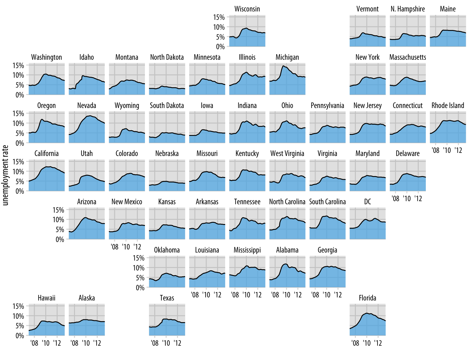
Cartogram

Use approximate geographical position to encode information, but not lat/long directly
Chloropleth Maps in detail

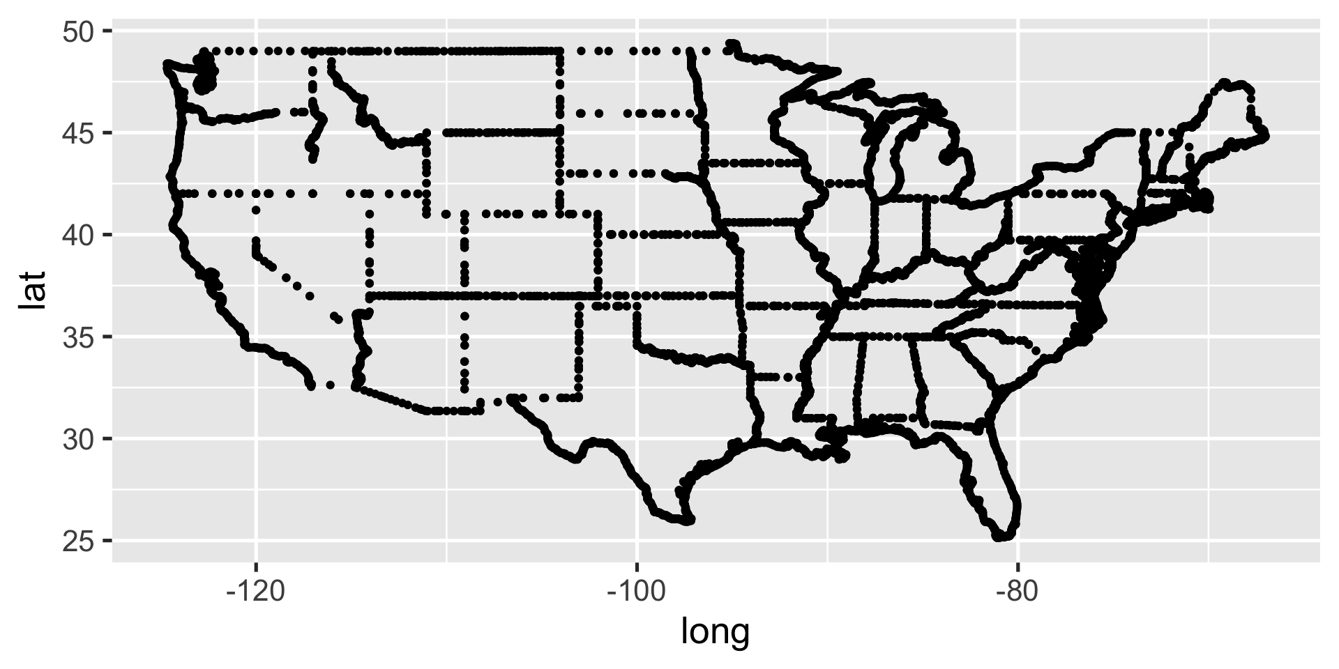
What is a map?

A bunch of latitude longitude points…
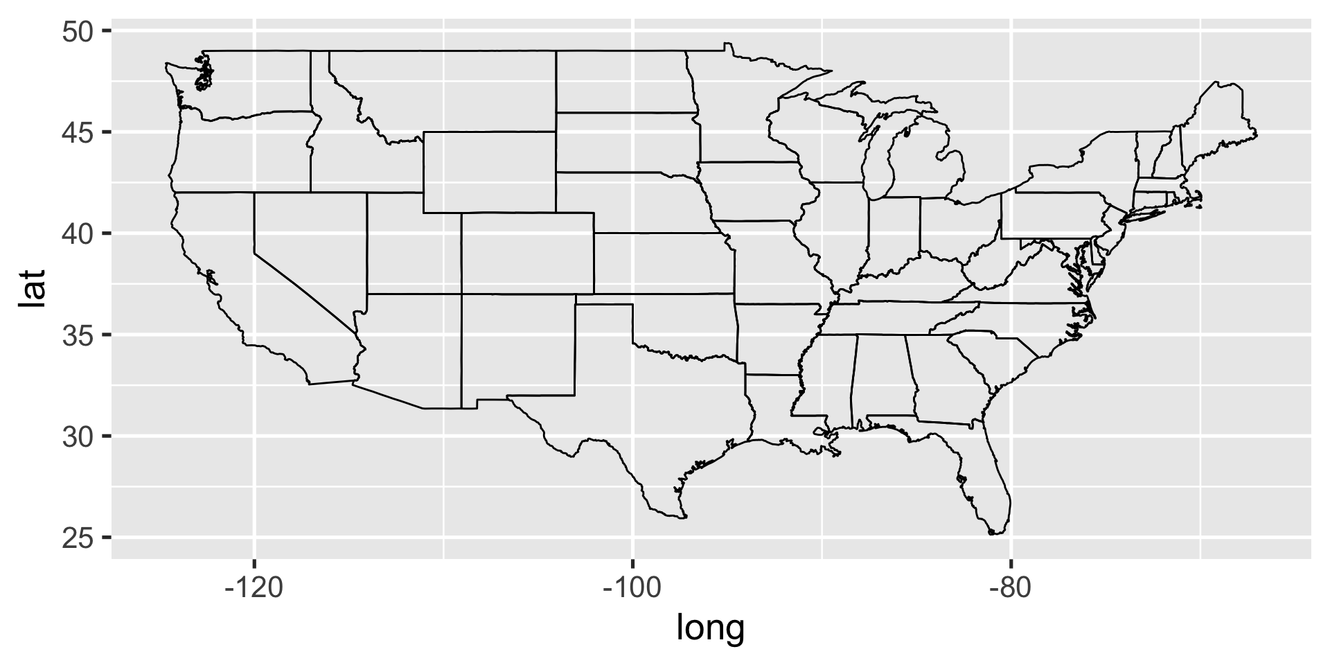
What is a map?

… that are connected with lines in a very specific order.
Necessary map data

  • latitude/longitude points for all map boundaries

  • which boundary group all lat/long points belong

  • the order to connect points within each group

State map data

ggplot2::map_data() provides the necessary information

states <- map_data("state")
head(states)
       long      lat group order  region subregion
1 -87.46201 30.38968     1     1 alabama      <NA>
2 -87.48493 30.37249     1     2 alabama      <NA>
3 -87.52503 30.37249     1     3 alabama      <NA>
4 -87.53076 30.33239     1     4 alabama      <NA>
5 -87.57087 30.32665     1     5 alabama      <NA>
6 -87.58806 30.32665     1     6 alabama      <NA>

Using geom_polygon()

Using geom_polygon() will treat states as solid shapes, making it easier to add color
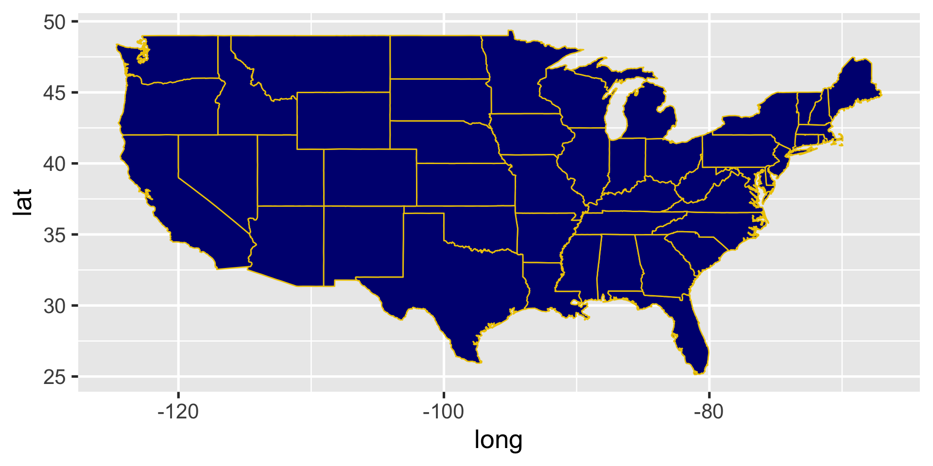
ggplot(states, aes(x=long, y=lat, group=group)) + 
    geom_polygon(color="gold2", fill="navyblue")

Using coord_fixed()

Using coord_fixed() forces x and y units to be equal
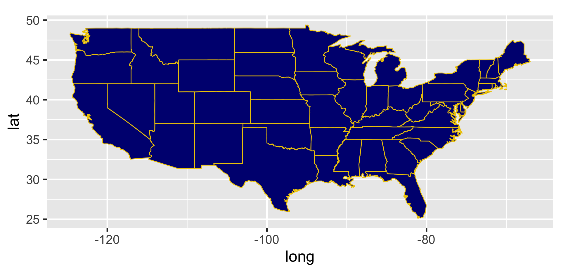
ggplot(states, aes(x=long, y=lat, group=group)) + 
    geom_polygon(color="gold2", fill="navyblue") +
  coord_fixed()

Your turn

ggplot(states, aes(x=long, y=lat, group=group)) + 
    geom_polygon(color="gold2", fill="navyblue") +
    coord_fixed()
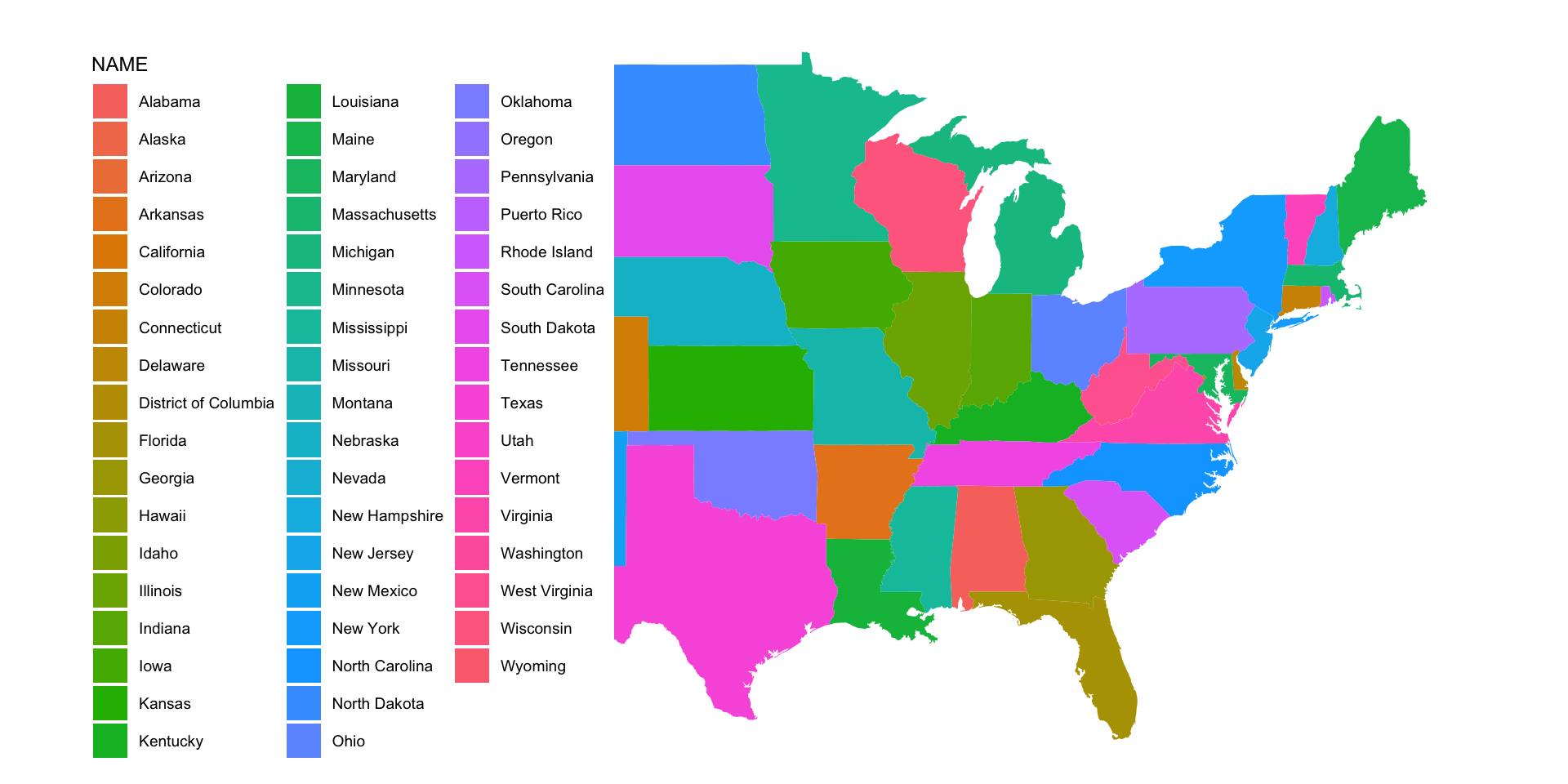
  • Edit this code so that each shape is colored in with a different color.
  • You only need the 3 variables used: long, lat, and group
  • 05-maps.qmd is available on the website
03:00

But… how do we include data?

acs_state_data = read_csv("https://raw.githubusercontent.com/aluby/teaching-datasets/refs/heads/main/acs_state_data_2022_5y.csv") 
acs_state_data$state = tolower(acs_state_data$NAME)
NAME med_age total_pop race_white race_black_afam race_am_indian race_asian race_hawaiian_pi race_other race_two_plus born_in_state male_age_married fem_age_married hs_diploma associate_degree bachelors_degree masters_degree prof_degree doctorate_degree med_income internet_any internet_dialup internet_broadband state
Alabama 39.3 5028092 3329012 1326341 21122 69808 93924 185632 63576 3454217 28.8 27.0 864977 306021 572252 261039 56574 42980 59609 1625807 6090 1619717 alabama
Alaska 35.3 734821 450472 23395 104957 47464 14597 82727 15138 314011 29.5 26.6 114087 43357 93744 39645 9589 6419 86370 236875 610 236265 alaska
Arizona 38.4 7172282 4781702 327077 297590 240642 549361 961794 668727 2849262 30.3 28.2 953769 445866 958447 429317 93897 69793 72581 2448838 5550 2443288 arizona
Arkansas 38.4 3018669 2193348 456693 16840 47413 89782 203476 106205 1843313 27.3 26.0 573876 159514 317437 134754 29822 19966 56335 968272 2584 965688 arkansas
California 37.3 39356104 18943660 2202587 394188 5949136 6388999 5327003 3506890 22254935 31.3 29.6 4837641 2136258 5935292 2515475 687281 488925 91905 12195945 18361 12177584 california
Colorado 37.3 5770790 4393409 233712 57022 185431 283146 609976 375060 2411879 30.2 28.2 660933 334723 1083618 481793 100044 76234 87598 2095757 4374 2091383 colorado
Connecticut 40.9 3611317 2522166 385407 9043 170945 233926 288485 162640 1945920 31.2 29.9 570708 192167 573917 341203 81685 46421 90213 1272555 2700 1269855 connecticut
Delaware 41.4 993635 634244 218266 3309 40570 32751 64130 28821 435760 30.7 29.3 184812 58540 139213 75033 13180 13931 79325 352105 673 351432 delaware
District of Columbia 34.8 670587 265633 297101 2209 27067 30879 47278 20539 241127 31.9 30.9 61269 14834 124860 109410 48095 21167 101722 281424 292 281132 district of columbia
Florida 42.4 21634529 13807410 3355708 59197 609990 1045557 2743467 2089692 7745873 31.0 29.1 3671306 1567030 3154240 1308569 372331 202326 67917 7429632 12312 7417320 florida
Georgia 37.2 10722325 5820019 3373948 37920 465487 378659 638881 315042 5796529 30.1 28.0 1611827 594639 1464589 669304 165134 108680 71355 3468542 4515 3464027 georgia
Hawaii 39.9 1450589 333296 28665 4210 538970 24503 370148 23091 769824 30.1 28.8 244486 113060 227243 85984 25539 16217 94814 435393 862 434531 hawaii
Idaho 36.9 1854109 1574859 12781 22297 24987 83887 132577 73263 830194 27.1 25.7 259629 119611 244372 85760 20684 15407 70214 608097 1915 606182 idaho
Illinois 38.7 12757634 8388659 1774605 55819 738071 842553 952451 606350 8549361 30.8 29.2 1899480 727981 1924339 938097 214115 130899 78433 4388839 9493 4379346 illinois
Indiana 38.0 6784403 5426227 640752 12465 168899 187740 345830 153259 4585916 29.2 26.8 1258288 408878 815853 342003 69602 52190 67173 2307571 6131 2301440 indiana
Iowa 38.4 3188836 2769619 120619 10111 78940 54569 150396 65729 2232446 29.1 26.9 568254 255181 433380 148289 36031 27629 70571 1117760 4880 1112880 iowa
Kansas 37.1 2935922 2341473 163581 22015 88513 102461 215150 96078 1740100 28.6 26.5 415315 171665 417263 185313 38167 27522 69747 1012599 2444 1010155 kansas
Kentucky 39.1 4502935 3816997 360184 6821 69187 56352 189589 68088 3069011 28.4 26.5 806274 269411 478134 241185 56939 35681 60183 1518043 4050 1513993 kentucky
Louisiana 37.6 4640546 2758714 1464582 24952 80363 84387 225187 98242 3604534 30.0 28.2 854193 215867 519481 206717 56332 33039 57852 1467429 2486 1464943 louisiana
Maine 44.8 1366949 1261284 21775 6722 15071 8128 53704 21246 835553 29.9 28.6 261945 103134 214733 90861 22065 15603 68251 509099 2409 506690 maine
Maryland 39.1 6161707 3154247 1841926 18343 399736 355402 388933 153723 2910096 31.1 29.5 885579 292090 952916 590587 135879 119364 98461 2103025 3649 2099376 maryland
Massachusetts 39.8 6984205 5075525 498785 14740 487600 347501 557288 322753 4151655 31.3 30.3 990524 374880 1234320 717317 153045 154129 96505 2489302 4031 2485271 massachusetts
Michigan 39.9 10057921 7617085 1363539 45662 327551 157999 543305 209757 7676334 30.4 28.5 1694166 673750 1311608 627217 132170 89356 68505 3529341 8375 3520966 michigan
Minnesota 38.5 5695292 4537219 382082 51434 286146 133098 302989 102874 3838865 30.1 28.3 800667 452032 965593 364292 89655 60300 84313 2030598 6584 2024014 minnesota
Mississippi 38.1 2958846 1685024 1101836 12777 29041 41764 87204 29813 2112621 28.7 27.0 468731 209117 286132 131671 30003 22265 52985 899120 1842 897278 mississippi
Missouri 38.8 6154422 4884165 693892 17559 127044 91703 331228 134401 4069809 28.8 27.0 1087681 345329 804597 370034 80507 54700 65920 2133965 5791 2128174 missouri
Montana 40.1 1091840 943827 6026 63493 9211 11592 57010 19231 578621 29.7 26.9 175154 72238 170549 59333 15762 11983 66341 386840 2330 384510 montana
Nebraska 36.9 1958939 1603239 93555 18550 48874 69315 124088 63635 1266893 28.7 26.7 280742 139287 280101 106137 25032 18160 71722 688362 2326 686036 nebraska
Nevada 38.5 3104817 1732783 290223 40745 263063 360620 395499 234103 846922 30.6 28.7 503894 186225 371761 139842 37727 22673 71646 1034261 1614 1032647 nevada
New Hampshire 43.1 1379610 1241594 20920 2070 36352 15009 63317 29967 565581 30.9 29.0 229881 100541 236189 116378 19939 16942 90845 497411 1295 496116 new hampshire
New Jersey 40.0 9249063 5528604 1213265 29780 913364 768606 792890 536450 4749727 31.1 29.6 1511209 430063 1636308 785250 182433 111577 97126 3119172 4904 3114268 new jersey
New Mexico 38.6 2112463 1250614 44894 198140 34400 233978 348588 278356 1139587 30.4 27.4 305319 128685 230705 131594 26832 27773 58722 666625 2368 664257 new mexico
New York 39.3 19994379 11749652 3011116 93384 1767598 1878496 1485013 883505 12567731 31.6 30.2 2933147 1238616 3033763 1731771 435559 238322 81386 6719878 13718 6706160 new york
North Carolina 39.1 10470214 6800458 2192455 109600 325670 421954 613129 278960 5747122 29.8 28.0 1505077 720557 1533552 648712 139534 107092 66186 3576483 6096 3570387 north carolina
North Dakota 35.4 776874 656425 25233 36284 12474 10705 34294 10445 483341 29.3 27.1 111395 72298 113131 33064 7189 5710 73959 275251 526 274725 north dakota
Ohio 39.6 11774683 9281702 1449450 17094 283278 157485 581637 190279 8810980 30.0 28.2 2315749 715379 1515763 696826 148249 98487 66990 4205747 10363 4195384 ohio
Oklahoma 36.9 3970497 2716667 284453 298628 91720 124427 447289 118519 2392787 28.1 26.2 674369 217129 465739 177413 42157 29429 61364 1306391 2678 1303713 oklahoma
Oregon 39.9 4229374 3328095 79593 46880 187852 180534 389281 168170 1932284 30.4 28.5 542883 272990 654185 283031 72199 54744 76632 1526087 4533 1521554 oregon
Pennsylvania 40.8 12989208 10010379 1407814 20570 473192 405422 667575 303356 9262753 30.7 29.1 2710001 805392 1844355 884422 199768 152773 73170 4540914 15090 4525824 pennsylvania
Rhode Island 40.1 1094250 816308 67615 4072 37881 75669 91944 56475 607146 31.6 30.2 173104 63413 165487 80811 19272 14255 81370 386033 648 385385 rhode island
South Carolina 40.0 5142750 3342861 1326209 15617 85834 123269 246238 103873 2787554 29.6 28.3 853211 357618 674340 305597 62767 46066 63623 1723516 3209 1720307 south carolina
South Dakota 37.5 890342 731624 19525 70948 12754 10567 44430 13890 560609 29.1 26.5 148100 72002 123313 38604 10123 6821 69457 305608 934 304674 south dakota
Tennessee 38.9 6923772 5182736 1126815 14118 128630 139938 326851 140517 4041432 28.8 27.3 1232458 367186 889401 368384 89488 66397 64035 2331002 4167 2326835 tennessee
Texas 35.2 29243342 17293460 3552579 169576 1511069 2281525 4407783 3547610 17298277 29.4 27.3 3792935 1435330 3919003 1598654 341512 242618 73035 9286171 12094 9274077 texas
Utah 31.4 3283809 2705194 37712 32948 77761 174721 224725 114101 2017569 26.8 24.9 383506 194933 468541 173551 36570 29475 86833 979140 2201 976939 utah
Vermont 42.9 643816 594131 8000 1336 10824 3568 25809 9039 311028 30.8 29.2 112763 39344 111614 57539 12438 9939 74014 230509 1620 228889 vermont
Virginia 38.7 8624511 5473610 1630355 23728 591088 303247 596298 252261 4245322 30.2 28.3 1184055 461866 1366160 780607 158770 119285 87249 2923674 6070 2917604 virginia
Washington 38.0 7688549 5374874 301477 91698 708647 399571 759279 292781 3584329 30.1 27.8 957379 541092 1244437 569699 123220 92087 90325 2749145 5275 2743870 washington
West Virginia 42.6 1792967 1639342 61227 1730 13602 9504 66905 22651 1225247 29.7 27.3 421521 101487 171758 84486 18450 14085 55217 594366 2333 592033 west virginia
Wisconsin 39.9 5882128 4854979 363331 43759 169052 128690 320056 155464 4165197 30.3 28.3 1071376 451044 852632 319419 70555 53667 72458 2137129 8839 2128290 wisconsin
Wyoming 38.5 577929 504798 4891 12359 4717 16504 34024 17046 245999 27.7 25.8 88797 46082 71313 31053 6077 5138 72495 207049 549 206500 wyoming
Puerto Rico 43.7 3272382 1425431 286388 5066 6295 786315 762608 600716 NA 33.8 32.4 617845 271432 482139 134673 30748 30891 24002 892631 14210 878421 puerto rico

geom_map is a “shortcut”

ggplot(acs_state_data) + 
  geom_map(
    aes(map_id = state, fill = NAME),
    map = states
  ) +
  expand_limits(x = states$long, y = states$lat) +
  coord_map() +
  theme_map()
  • acs_state_data is the name of the dataset
  • map_id = state tells geom_map to look in the “state” column in acs_state_data to find the state name
  • fill = NAME tells ggplot to fill the states by the variable in NAME

geom_map is a “shortcut”

Your turn 1

Comment out the expand_limits line. What happened?

01:00

Sequential vs Diverging color scale

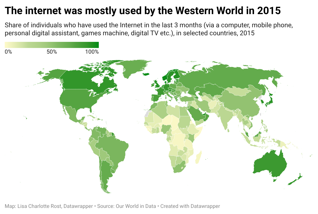
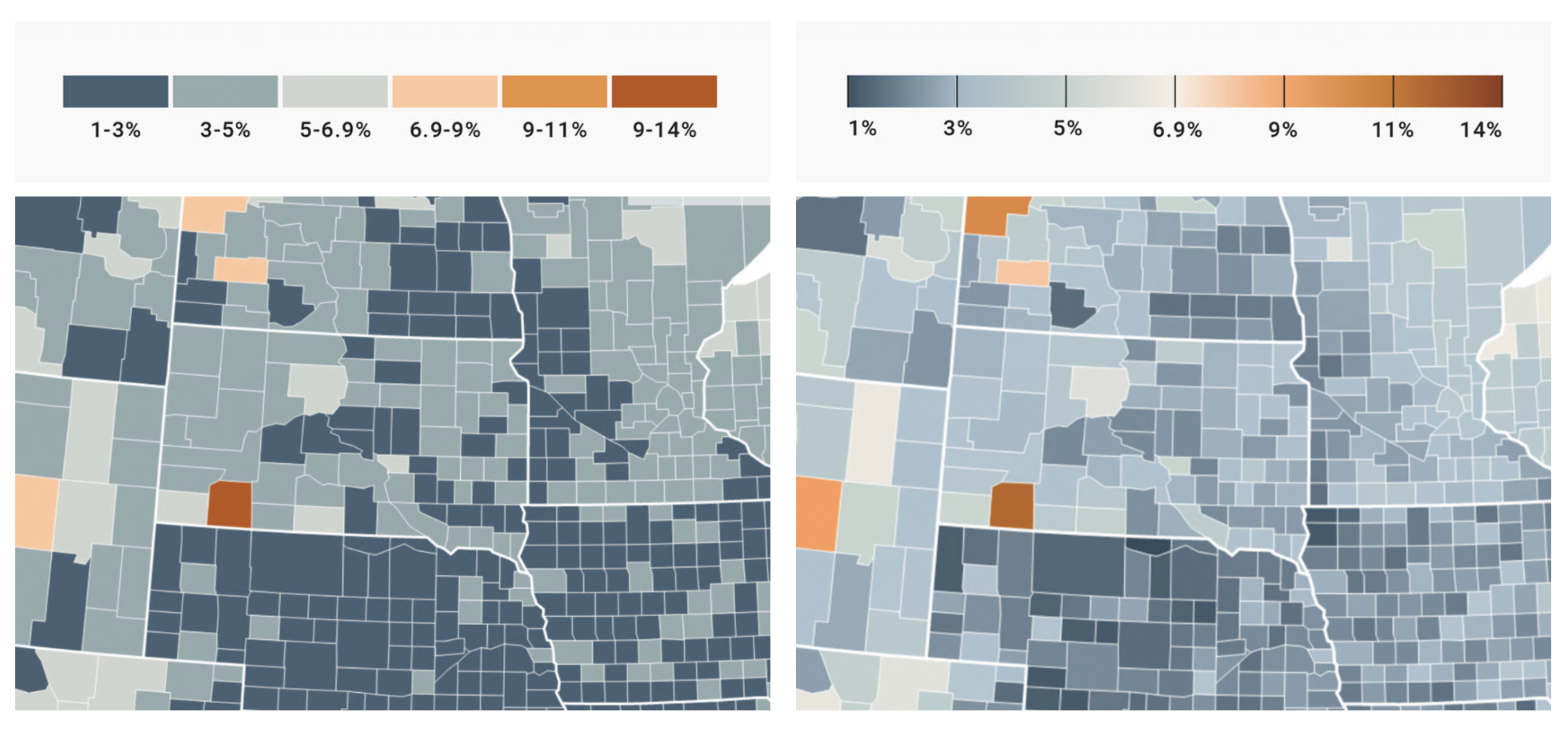
The next two panels show the same data and the same graph with two different color scales.

Sequential color scales are intuitive and can be read as “more is more”

Diverging scales emphasize how far away a data point is from a midpoint
Binned vs continuous color scale
Your turn 2

Edit your chloropleth map by:

  • Choosing a different variable in acs_state_data to map to fill
  • Choosing a different color scale
  • Updating the title, axis labels, and legend title
06:00

Coordinate Systems and Projections

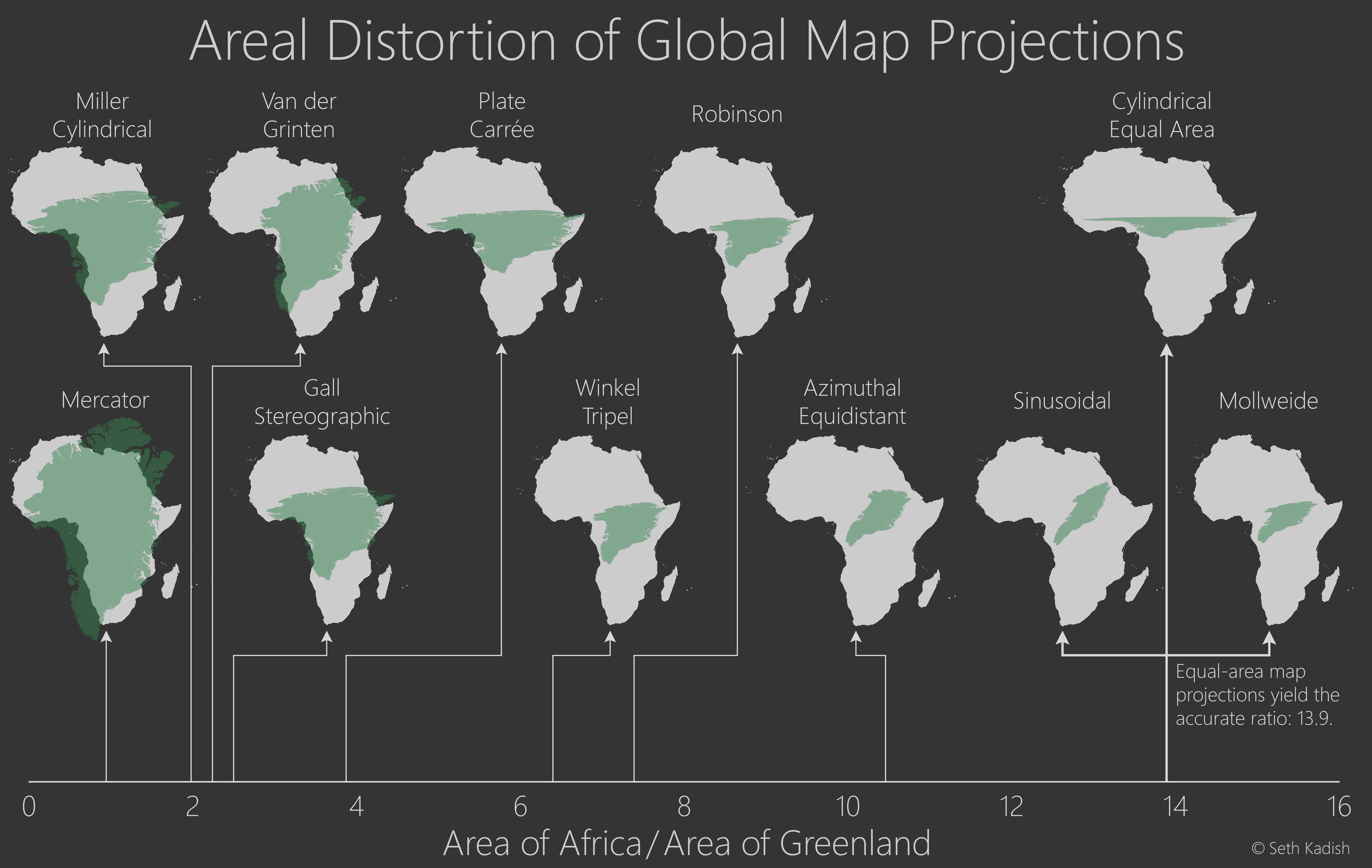
Geospatial data exists on the globe and is generally described with a latitude and longitude. Any projection from the globe to euclidean space (X-Y plane) is going to cause some distortion.

Changing the coordinate system

coord_map function provides a Mercator projection (mapproj package has more options)
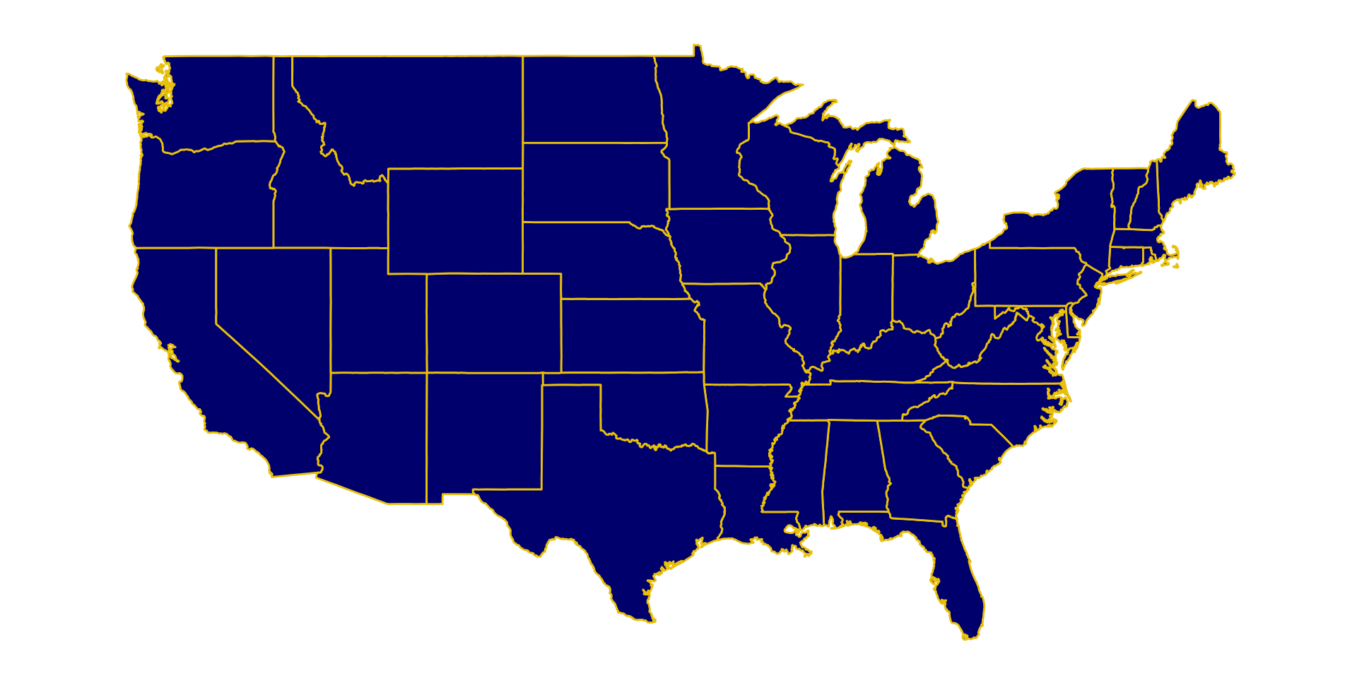
ggplot(states, aes(x=long, y=lat, group=group)) + 
  geom_polygon(color="gold2", fill="navyblue") + 
  coord_map() + 
  theme_map()

Changing the coordinate system

Here is a Gall projection
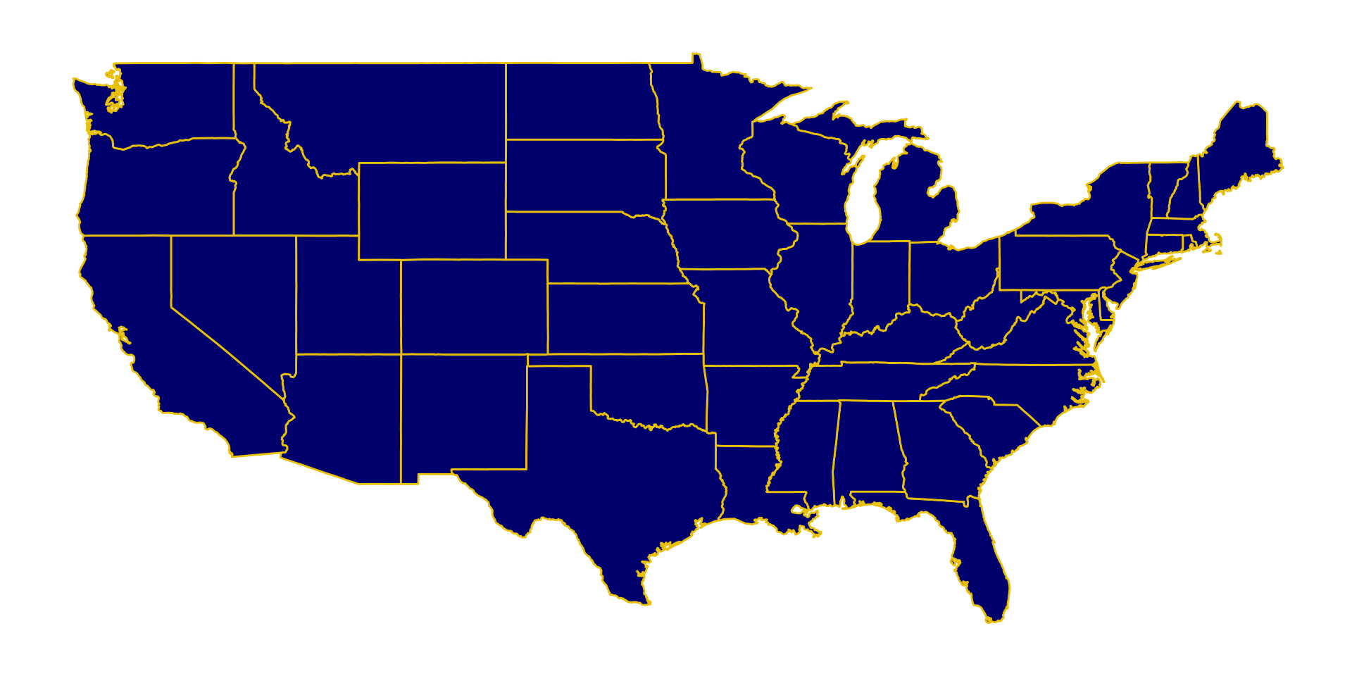
ggplot(states, aes(x=long, y=lat, group=group)) + 
  geom_polygon(color="gold2", fill="navyblue") + 
  coord_map(projection = "gall", lat = 0) + 
  theme_map()

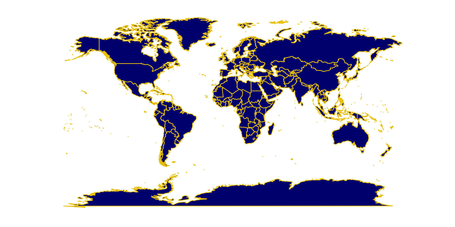
Mercator vs Gall projection (world map)
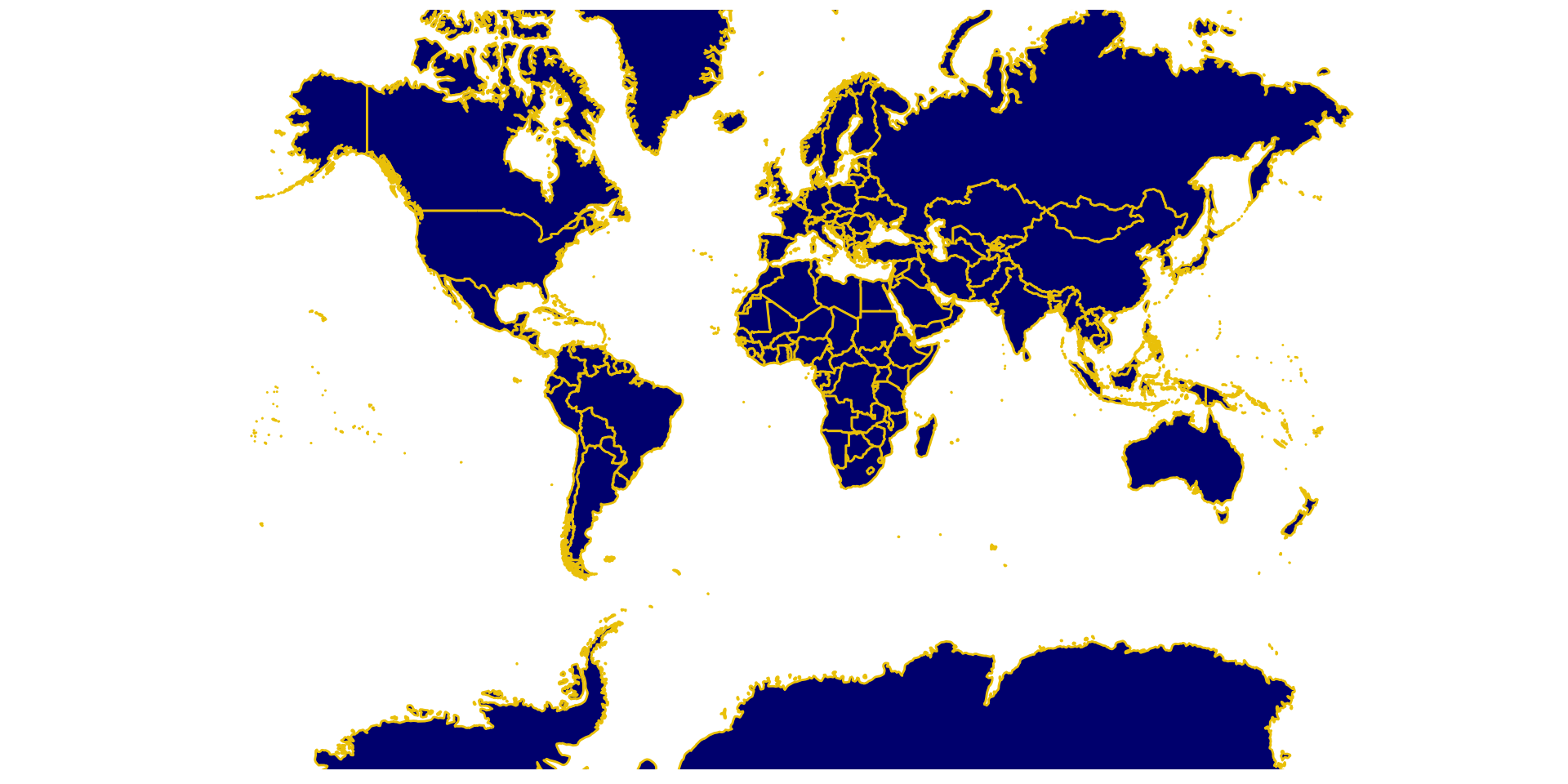
world <- map_data("world")

ggplot(world, aes(x=long, y=lat, group=group)) + 
  geom_polygon(color="gold2", fill="navyblue") + 
  coord_map(projection = "mercator", xlim = c(-180, 180)) + 
  theme_map()